personal
︎
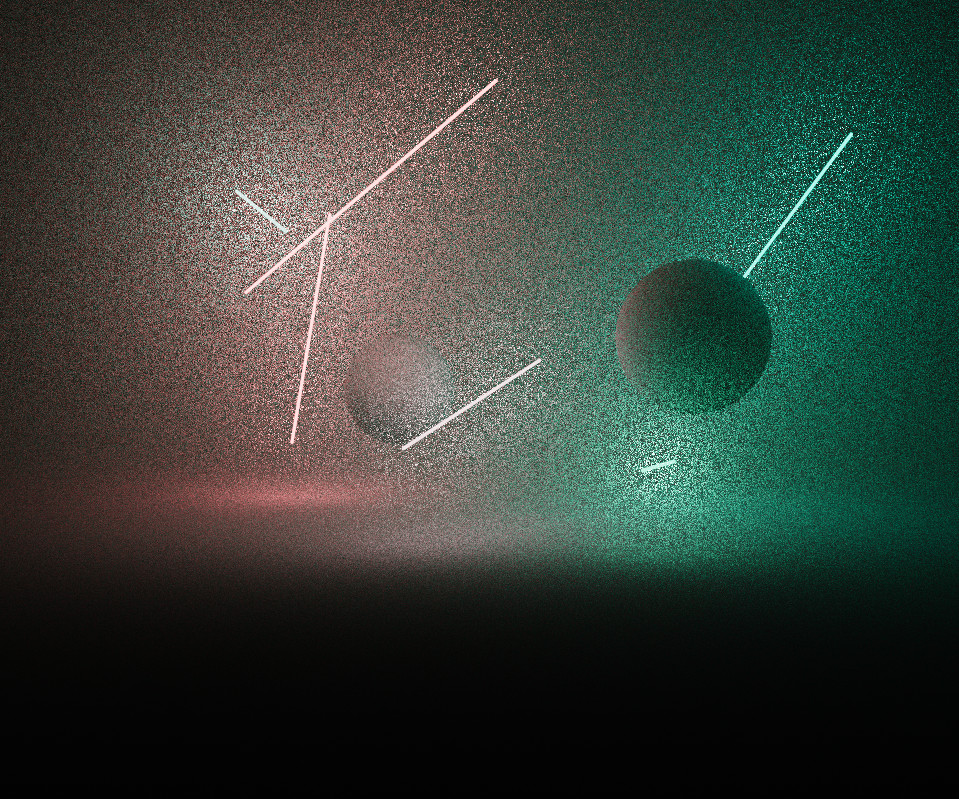
An iteration of the realtime generative system - mouse drag to explore
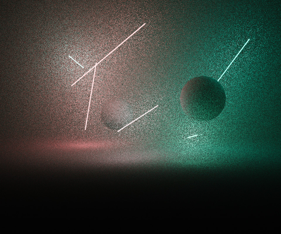
Wandering Nets
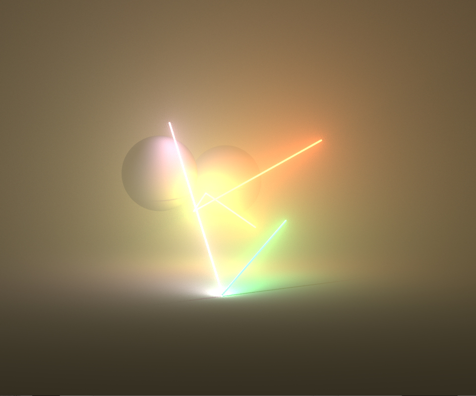
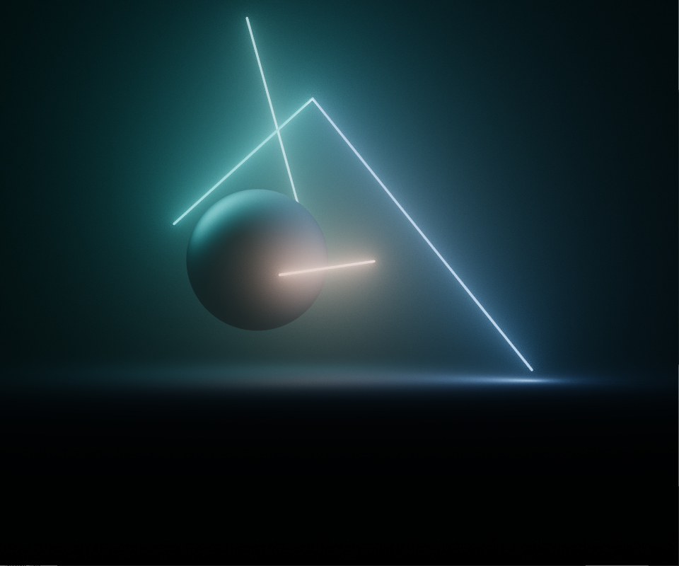
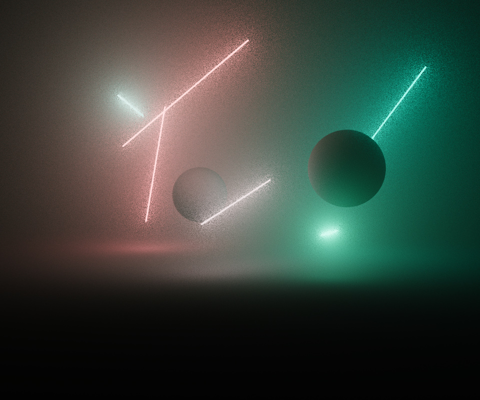
Wandering Nets is a generative art piece resulting from personal research and exploration in realtime volume rendering. Networks of light are created and connected via random walks in space and colour. Emergent structures are revealed by the ambient interaction, tension and collision of these networks within themselves and orbiting shadowed spherical bodies.
The piece runs in realtime in the browser using webgl. Scene data is generated and animated with Javascript and sent through to a single GLSL fragment shader, which renders the final pixels to a fullscreen quad. No external libraries are used, it’s a bespoke creation that’s tuned for purpose.
The piece runs in realtime in the browser using webgl. Scene data is generated and animated with Javascript and sent through to a single GLSL fragment shader, which renders the final pixels to a fullscreen quad. No external libraries are used, it’s a bespoke creation that’s tuned for purpose.
I’ve dabbled in OpenGL over the years for various purposes but this is the first fully realtime and interactive creative project I’ve executed. While my work often involves creative coding with procedural and generative techniques it’s usually complex, heavy and rendered using offline renderers, so it was both challenging and exciting to work in this medium.
The piece was released on fxhash, an online platform for generative art which allows users to generate and collect individual and unique iterations of code-based artwork - the edition contains over a hundred different outputs.
The piece was released on fxhash, an online platform for generative art which allows users to generate and collect individual and unique iterations of code-based artwork - the edition contains over a hundred different outputs.
Inspiration
My original idea was to create an atmospheric light sculpture, with colour radiating and mixing through fog. I wanted to take advantage of the realtime medium and create something dynamic, that would randomly, slowly unfold into different shapes and compositions over time. I’ve always been fascinated by the idea of fluorescent lights glowing on their own underneath high voltage power lines, energised by the magnetic field - this provided some inspiration but more interesting was the idea of a network of lights, with connectivity and interaction.
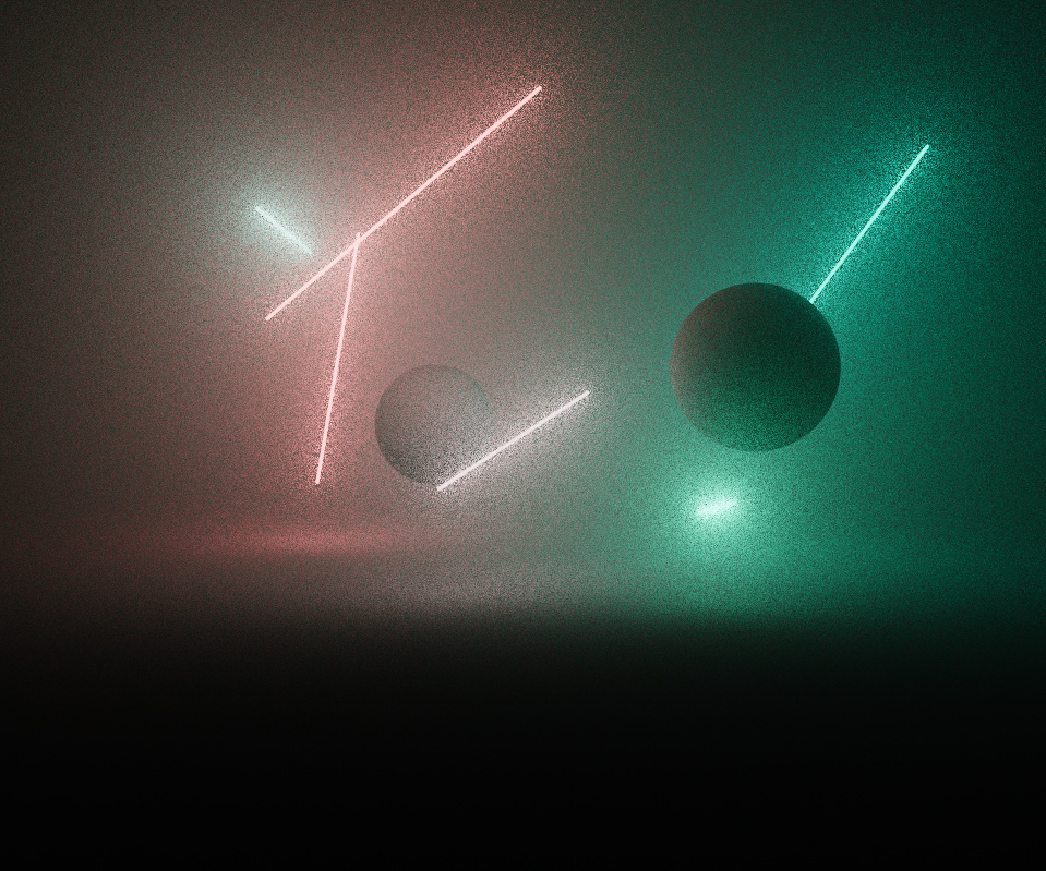
On their own the lights were interesting, but needed more of a sense of contrast, tension and rhythm. The circling orbs visually provide figure and ground, silhouette and shape, and heaviness in opposition to the lightness of the beams. This is the case not just in terms of visual composition, but in their animated behaviour - the lights collide and deflect off the orbs but the orbs are unaffected by the lights.
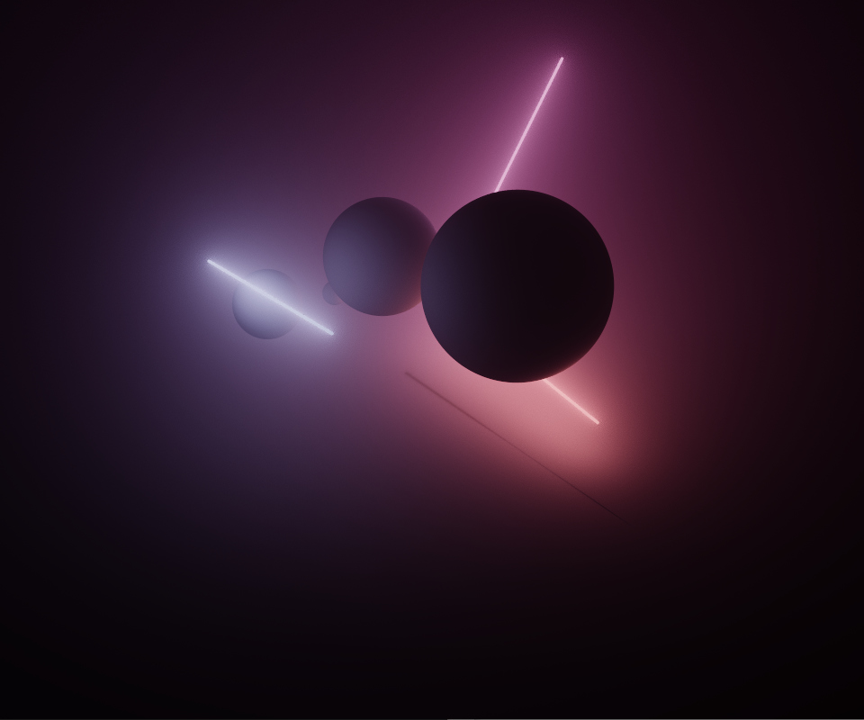
After a while, the scenes began to evoke an idea of constellations and planets, a kind of celestial diagram. This inspired the name Wandering Nets, referencing the original Greek planetes, meaning “wandering stars”.
After a while, the scenes began to evoke an idea of constellations and planets, a kind of celestial diagram. This inspired the name Wandering Nets, referencing the original Greek planetes, meaning “wandering stars”.
Variation
The light network structures are generated via a random walk process. Starting with a single point, edges are created and stored in a graph data structure. Each edge makes two different random decisions, for the first edge vertex it chooses to either:
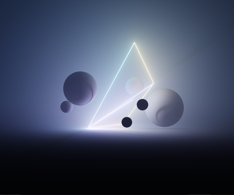
These rules create a range of different network topologies, from discrete disconnected segments, to chains of branching edges, and in the rarer cases, fully consolidated shapes such as a tetrahedron.
Additional variation is revealed by emergent behaviour in the networks’ animation. A simple semi-physically based physics simulation generates orbital motion. The connected networks are constrained by edge tensions, and collisions (between spheres ︎︎︎ lights and spheres ︎︎︎ spheres) which prevents interpenetration and contribute to unpredictability.
The parameters driving the animation and physics are randomised either per-element or per-iteration.
- Create a new starting point in space
-
Share an existing vertex in the graph and branch off
- Leave the endpoint floating freely, a random distance offset from the initial
- Connect the endpoint back to an appropriate existing point in the graph
These rules create a range of different network topologies, from discrete disconnected segments, to chains of branching edges, and in the rarer cases, fully consolidated shapes such as a tetrahedron.
Additional variation is revealed by emergent behaviour in the networks’ animation. A simple semi-physically based physics simulation generates orbital motion. The connected networks are constrained by edge tensions, and collisions (between spheres ︎︎︎ lights and spheres ︎︎︎ spheres) which prevents interpenetration and contribute to unpredictability.
The parameters driving the animation and physics are randomised either per-element or per-iteration.
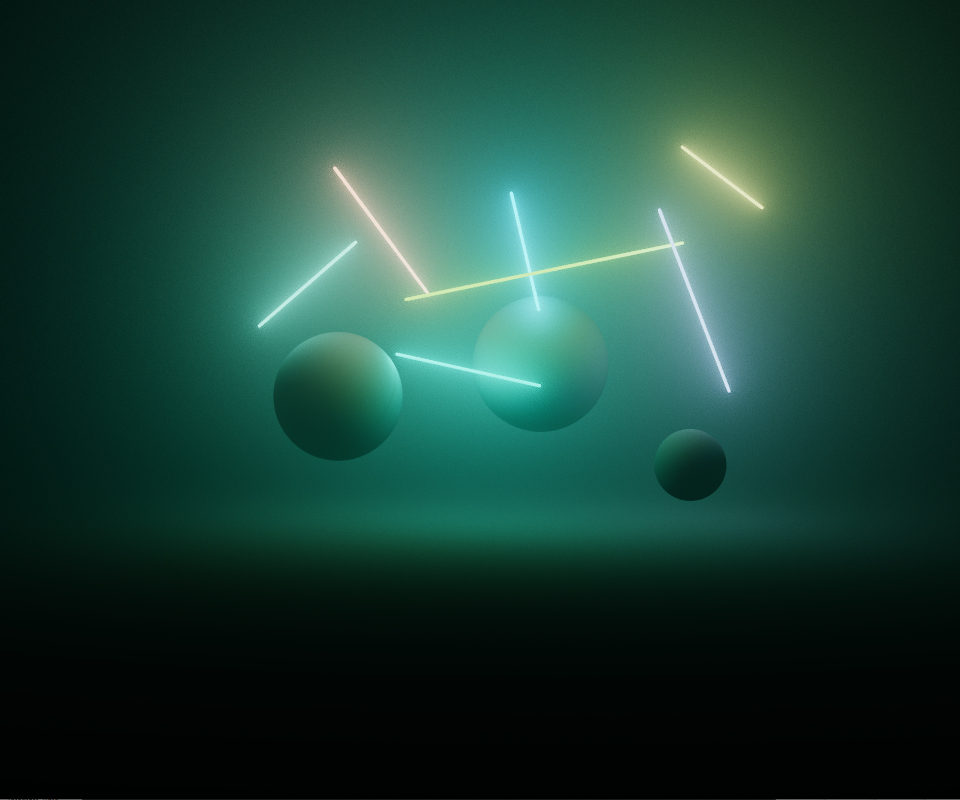
Colour schemes are also generated via a random walk process. For each edge in the graph, a random step is taken in the ab plane of the oklab colour space, to then be converted back to rgb. Randomly varying the size of the steps, or randomly constraining overall saturation gives a range of colour schemes varying between desaturated, monochromatic, or highly varied colour selections.
![Random walk in the ab plane]()

Features
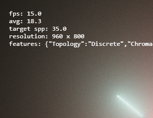
The fxhash platform has a concept of ‘features’: naming and grouping various traits to classify each individual unique iteration.
Rather than using features prescriptively, to set procedural parameters or presets used in the generative process, I found it more interesting to use them descriptively. When the scene data is first generated, with all the layers of randomisation involved, a secondary process then inspects the scene (i.e. analysing the generated network topology, or doing a simple statistical analysis on the colouring) to then describe what it found. I felt this allowed for a richer set of results than purely hard coding special cases.
Rather than using features prescriptively, to set procedural parameters or presets used in the generative process, I found it more interesting to use them descriptively. When the scene data is first generated, with all the layers of randomisation involved, a secondary process then inspects the scene (i.e. analysing the generated network topology, or doing a simple statistical analysis on the colouring) to then describe what it found. I felt this allowed for a richer set of results than purely hard coding special cases.
// ---- fxhash features

function f_topology(graph) {
    if (graph.points.length == 2*graph.edges.length)
        return "Discrete";

    if (graph.edges.some( ed => ed.points[0].edges.length == 1 &&
    	ed.points[1].edges.length == 1))
        return "Varied";

    if (graph.edges.length == 6 &&
    	graph.points.every( pt => pt.edges.length == 3 ))
        return "Tetra";

    if (graph.points.every( pt => pt.edges.length >= 2 ))
    	return "Consolidated";
    else
    	return "Branched";
}
Analysing topology to classify networks
Rendering Scene Data
The generation and animation of the lights is handled in Javascript using a simple adjacency list graph data structure. Since there are so few elements, speed is not a concern, but it’s mainly for convenience of manipulating and inspecting the network.
After each frame’s animation, the graph is converted to a simpler disconnected representation for rendering, with some common values pre-calculated. These are passed to the fragment shader as arrays of GLSL uniform structs.
Rays are then intersected from the camera position, against all the objects in these arrays to find the nearest shading point and normal. Volume lighting is calculated along the ray segment in between. Much of the primitive intersection code is derived from Inigo Quilez’s comprehensive examples.
struct Light {
	float intensity;
	vec3 colour;
	vec3 pa;
	vec3 pb;
	float w;
	vec3 L;
	vec3 nL;
};

struct Sphere {
	float r;
	vec3 P;
};

#define MAX_LIGHTS 20
uniform int u_numLights;
uniform Lights
{
    Light lights[MAX_LIGHTS];
};

#define MAX_SPHERES 6
uniform int u_numSpheres;
uniform Spheres
{
    Sphere spheres[MAX_SPHERES];
};
GLSL Uniforms
Volumes
Rendering volumes in realtime is challenging, and it’s been a while since I’ve worked on developing a volume renderer, so I wanted to use up to date techniques. The biggest challenge was getting it to be performant without compromising too much on the level of visual quality I wanted. Optimising it involved two main strategies:
- Being smart (using effective sampling strategies optimised for low sample counts)
- And being dumb (hacking and cheating to avoid spending cycles where they won’t be noticed)
The dumb part is mostly about avoiding work wherever I could get away with it. For example:
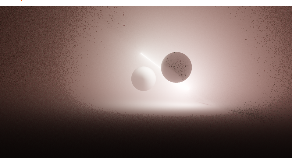
![Undersampled shadow regions (exposed up x8)]()
- Limiting pixel samples in dark areas - after taking a few samples from each light, if a pixel is still dark it stops taking further samples. If you expose up you can see noise in the shadows but it’s not noticable at normal brightness.
- Not bothering to send visibility rays if the remaining terms of the rendering equation components of the current sample’s rendering equation will provide low radiance anyway (eg. geometric term/inverse square falloff/pdf)
Light Sampling
Sampling lighting in thin volumes requires specific strategies. Sampling at every step as in a naive ray marcher is slow and wasteful, importance sampling according to extinction is ineffective since extinction due to density is not the dominant term. However a highly effective sampling strategy is equiangular sampling, presented by Christopher Kulla (Sony Imageworks) which samples lighting in the volume at distances proportionally to where light contribution is the strongest. It’s essentially sampling proportionally to the solid angle projection of the viewing ray, on the sphere around the light source.
Although the technique was originally intended for use with point lights, it extends to other shapes - first find a sample location on the emitter, then use equiangular sampling to find a distance along the ray to sample lighting (with optional MIS for areas where the chosen location on the light is suboptimal)
Although the technique was originally intended for use with point lights, it extends to other shapes - first find a sample location on the emitter, then use equiangular sampling to find a distance along the ray to sample lighting (with optional MIS for areas where the chosen location on the light is suboptimal)
Rather than just specifically for distance sampling in a volume, equiangular sampling can be thought of as a generic method for importance sampling a line segment relative to the solid angle as seen from a point. I found it’s possible to reuse this technique in other situations that I haven’t yet seen documented - one example is flipping it around to importance sample line lights from single shading points on solid geometry. I’ve added a simple demonstration of this on shadertoy:
Importance sampling line by solid angle from surface shading point
Another potential use case might be in initially sampling a position on a line light relative to the view ray, before then sampling a distance along the ray. By projecting the line light against the plane defined by the view ray, we can collapse the ray into a single point, giving us a point-line segment relationship where we can sample by solid angle using the same techniques. After finding a position along the light line segment in projected space, we can then map that back to the original light to find a sample position in 3D.
The end result is that areas on the light source close to the ray are sampled more densely than areas further from the ray, concentrating work where it will have more of an effect on the final radiance.
This works well for infinite rays, but for clipped view rays (eg. if there is an occluding object) it reveals artifacts. This makes sense since if there is a light further beyond the end of the clipped ray, the solid angle projection is different to how it would be it it was more ‘perpendicular’ to a long/infinite ray, as this technique assumes. In the end, while promising, I didn’t find a solution for these artifacts so didn’t end up using it for this project. I think there’s potential though, so if anyone smarter than me has ideas, please take a look at the shadertoy and share your thoughts.
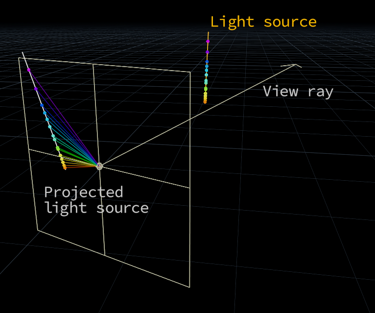
Importance sampling line by solid angle from collapsed view ray
(Quasi) Random Sequences
Raytracing/pathtracing requires liberal use of random numbers. In this case, for each pixel sample choosing:
Often better than pure random numbers are low-discrepancy (quasi-random) sequences. These still exhibit similar properties to random numbers, but with a more even distribution that reduces noise. The last time I looked deeply into low-discrepancy sequences was about a decade ago; since then Martin Roberts has presented the quite brilliant R-sequence, which is simple and with many desirable qualities.
I initially substituted the R-sequence in place of a random hash function, resetting/offsetting into the R-sequence for each pixel, and stepping through the sequence for each pixel sample. Because the sequence was getting randomly disconnected between pixels, it was not giving that much better results than a pure random hash.
Due to the way new samples cover the domain by filling in the areas between existing samples, when randomly indexing you might get adjacent pixels utilising parts of the sequence with similar patterns. This will introduce noise if you get ‘clumping’ of results, i.e. a few adjacent pixels which sampled bright areas on a light clumping together.
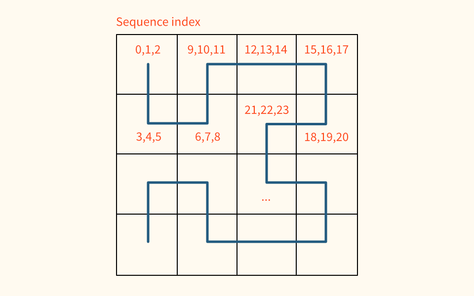
I’d seen examples of people using the R1 sequence for dithering. Rather than a random offset into the sequence per pixel, one can use the index of a space filling curve like the Hilbert curve as it covers the pixel grid. This takes advantage of spatial coherence - nearby pixels will get adjacent indices in the R1-sequence, which will be evenly distributed and reduce noisy clumping.
- A ray offset for antialiasing
- A light to use
- A position on the light
- A distance along the view ray to sample radiance
Often better than pure random numbers are low-discrepancy (quasi-random) sequences. These still exhibit similar properties to random numbers, but with a more even distribution that reduces noise. The last time I looked deeply into low-discrepancy sequences was about a decade ago; since then Martin Roberts has presented the quite brilliant R-sequence, which is simple and with many desirable qualities.
I initially substituted the R-sequence in place of a random hash function, resetting/offsetting into the R-sequence for each pixel, and stepping through the sequence for each pixel sample. Because the sequence was getting randomly disconnected between pixels, it was not giving that much better results than a pure random hash.
Due to the way new samples cover the domain by filling in the areas between existing samples, when randomly indexing you might get adjacent pixels utilising parts of the sequence with similar patterns. This will introduce noise if you get ‘clumping’ of results, i.e. a few adjacent pixels which sampled bright areas on a light clumping together.
I’d seen examples of people using the R1 sequence for dithering. Rather than a random offset into the sequence per pixel, one can use the index of a space filling curve like the Hilbert curve as it covers the pixel grid. This takes advantage of spatial coherence - nearby pixels will get adjacent indices in the R1-sequence, which will be evenly distributed and reduce noisy clumping.
All the instances of this technique that I’d seen though, only dealt with a single sample per pixel, so I sketched out some tests on shadertoy with various ways of combining/averaging results from multiple samples per pixel.
The best results came from continuing the sequence ‘through’ the pixel, incrementing the sequence offset for each pixel sample before continuing on to the next hilbert index.
![Example R1 sequence indices through Hilbert curve, 3 samples per pixel]()
In the case of line lights, I found more improvements in not continuing the sequence through all pixel samples, but separately for each light. This ensured a well distributed set of sampled positions along each emitter, rather than the sequence being scattered across multiple lines. This is implemented with an array of sample counters (one for each light), incremented each time a light is sampled, and then used to calculate the sequence index.
The best results came from continuing the sequence ‘through’ the pixel, incrementing the sequence offset for each pixel sample before continuing on to the next hilbert index.
In the case of line lights, I found more improvements in not continuing the sequence through all pixel samples, but separately for each light. This ensured a well distributed set of sampled positions along each emitter, rather than the sequence being scattered across multiple lines. This is implemented with an array of sample counters (one for each light), incremented each time a light is sampled, and then used to calculate the sequence index.

Performance
Being presented in a realtime web based medium, there’s little control over the viewing environment. I wanted to ensure that it would remain as fluid as possible, and true to intention on a range of different devices. By default the sampling rate is automatically adjusted to attempt to maintain as close as possible to 30 frames per second playback. A running average of fps is taken - if it is too low, it reduces the number of samples per pixel, otherwise it increases sampling to maximise visual quality. This allows the piece to be functional at a lower level of visual quality even on devices like phones.
Colour
I wanted the piece to support very intense levels of saturation with a robust colour process. The image is rendered in a linear wide gamut ACEScg AP1 working space, and is converted to sRGB after merging pixel samples. I’m used to working in this colour space anyway, so it was a natural fit.
It was important for the intensity and gradation of light to be faithfully reproduced without clipping, so doing a simple gamma 2.2 sRGB approximation was out of the question. Initially I used a polynomial fit approximation of the ACES RRT tone mapping curve, but was suffering from colour skew and gamut clipping as the rgb ratios were scaled non-linearly, especially with bright and highly saturated lights.
It was important for the intensity and gradation of light to be faithfully reproduced without clipping, so doing a simple gamma 2.2 sRGB approximation was out of the question. Initially I used a polynomial fit approximation of the ACES RRT tone mapping curve, but was suffering from colour skew and gamut clipping as the rgb ratios were scaled non-linearly, especially with bright and highly saturated lights.
An experiment from Björn Ottosson provided a solution, which I borrowed with permission - it converts the final colour to his Oklab space and performs the tone mapping there, weighted by the derivative of the tonemap curve. It does a great job of preserving the correct hue and desaturates out of gamut colours, giving a more filmic colour response.
The below images demonstrate the effectiveness - even though the per-channel tone map is a lot better looking than the horribly clipped gamma 2.2, the colours skew, causing the redder lights to appear overly yellow.
The below images demonstrate the effectiveness - even though the per-channel tone map is a lot better looking than the horribly clipped gamma 2.2, the colours skew, causing the redder lights to appear overly yellow.